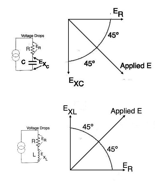
Now we have learned that there are two types of reactance: inductive and capacitive. With respect to the applied voltage, capacitive reactance polarity is opposite to the polarity of inductive reactance.
In the diagram above, we have the same diagram showing inductive reactance on the bottom we saw in the Inductance section of the blog but now with capacitive reactance on the top.
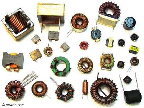
Another component that has a lot of variants is the inductor. Transformers are also a type of inductor that will be covered later in the Blog. Inductors are basically a coil of wire, however, that coil can be formed by many different techniques and wound around air, iron, ferrite, or plastic.
As we learned in the Magnetism section, when a DC voltage is applied to a wire, the wire radiates a magnetic field. When the wire was coiled around an iron core (such as a nail) a fairly strong magnetic field was created around the core and the nail acted as a magnet. Withdrawing the nail still left a magnetic field in place, though quite a bit weaker due to the removal of the highly permeable iron nail core.
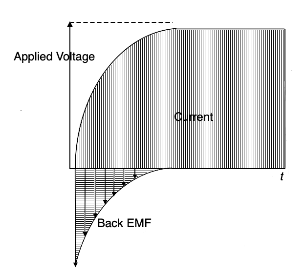
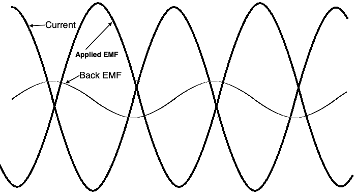
From the instant that current is applied to the wire or coil of wire, a magnetic field expands from the center of the conductor outward. As the magnetic field moves through the conductor, an opposing voltage is generated in the conductor (the same way that a conductor moving within a magnetic field creates voltage in a generator) in a direction that opposes the applied current. That generated voltage is called a “counter” EMF or “back” EMF. As the current comes to a steady state, the back EMF dissipates. That effect is shown in the diagram below. Although the effect is seen in straight conductors, the effect is greatly multiplied when the conductor is formed into a coil and still more when a conductive core is added to the center of the coil.
Recall from the section on capacitors that there is always a bit of a delay in the increase in charging voltage as current is applied (and a decrease in current flow as the maximum charge is reached). The main contributor to that delay was the series resistance (the R) in the time constant circuit, although ESR also contributed to the delay. Additionally, there is a slight amount of resistance in the wire in the coil that contributes to a similar effect in inductors as well.
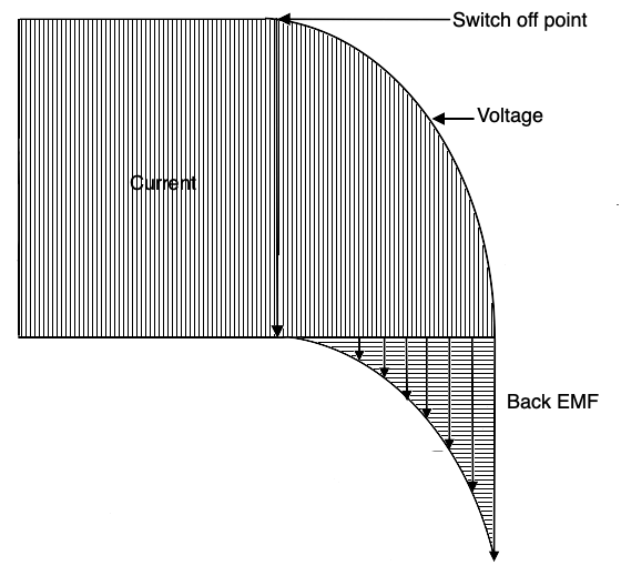
Now, just as when current begins flowing into an inductor it creates a back EMF due to the expanding magnetic field, when that current is removed, abruptly, like when a switch opens, the magnetic field collapses, and that movement of the field through the conductor again creates a back EMF. That may cause problems in a variety of circuits. In power grid circuits, that back EMF may cause spark jumps in distribution equipment potentially causing fires. It circuits carrying low voltage DC in relay contacts it may also cause sparking which could disrupt signals in adjacent circuitry. There are ways to mitigate these back EMF difficulties which will be discussed later. For now, be aware of the back EMF phenomenon that occurs as current is both applied and removed from an inductor.
In the illustration above we can see an exaggerated representation of an AC signal and the much reduced back EMF signal generated in an inductor.
Any change of current amplitude or direction in a conductor causes a back EMF which opposes the change of current flow. DC does not create a back EMF but varying DC and AC do. Inductance then is defined as the property that opposes the change in current or is the energy that is stored in an electromotive field. Inductance is measured in Henrys and an inductor is indicated by the symbol L. A single Henry is a huge amount of inductance, and like Farads with capacitance, we usually deal with millihenrys (mH) or microhenrys (uH or µH). The ability to oppose changes in current can be exploited to help smooth out power in power supplies and RF frequency circuits. When designed for these uses, they are called chokes because they choke off changes.
The inductance of a coil increases as the number of turns squared (N2). If there are 2 terns, the inductance is multiplied by 4 over a straight wire., 3 turns multiplies the value by 9, and so on. However, if the coils are spread out, the inductance decreases so the length of the coil comes into play. Also as the radius or diameter of the coil increases, more wire will be used and inductance will increase. A formula then that approximates the inductance is given by: L(µH) = r2N2 / 9r+10l where r is the coil radius in inches, N is the number of turns, and l is the length in inches.
Like capacitors, inductors can be combined with resistors to make a circuit that has a time constant. T = L/R (T is the time in seconds, L is the inductance in Henrys, and R is in ohms.
Inductance values in series and parallel combinations are computed just like resistances. L = L1+L2+L3 for inductances in series, and L = 1 / 1/L1+1/L2+1/L3 for inductances in parallel.
Referring to the illustration above, as the current increases through an inductor, the magnetic field also increases. At the moment that the current reaches its maximum, the rate of change drops to zero. As the current decreases toward zero, the magnetic field collapses inward to the conductor reaching a maximum positive or negative peak at the zero current point. Current leads applied voltage by 180º while induced back EMF lags current by 90º.
We have seen that DC flowing in an inductor has no dynamic effect, however AC does. As the current increases and decreases (let’s consider a steady state AC wave to begin with), the induced back EMF voltage resists the change. This resistance to change is called reactance. Inductive reactance, indicated by the symbol X, is a measure of how much the back EMF opposes the current change and is measured in ohms. A 1H inductor will have a specific reactance in a 60 Hz circuit while a 2H inductor will have twice as much reactance in the same circuit. Therefore, reactance is directly proportional to the inductance. The equation XL = 2πƒL where ƒ is the frequency in Hz, L is inductance in Henrys. 2πƒ is used so many times in electronics it has its own special symbol, ω. So, XL = ωL.
Reactance fits into Ohm’s Law equations just like R. So E = IXL, XL = E/I, I = E/XL. Additionally, inductive reactance in series or parallel circuits is computed just like resistance: XL: = XL1+XL2+XL3 for series circuits; XL = 1/1/XL1+1/XL2+1/XL3 for parallel inductances.
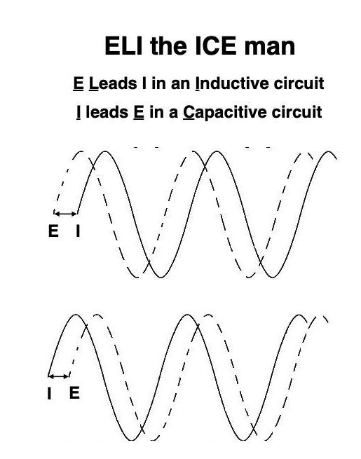
The illustration below shows E leading I in an inducative circuit while I leads E in a capacitive circuit. We can remember this difference with the nemonic “ELI the ICE man”. In all of the illustrations in the blog so far, we’ve had to represent the AC signal’s waveform as a steady state AC. In reality, that very rarely happens. Usually the AC signal is varying in amplitude . frequency, and phase at extremely high speeds making illustration impossible. For our purposes here, we are learning the basics, not trying to illustrate reality.
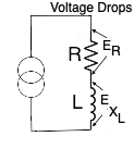
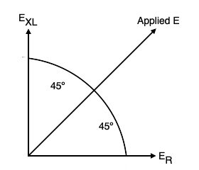
This next illustration shows an AC signal source along with a resistor (R), and an inductor (L). As we saw in the previous illustration, there are actually two voltages present in this circuit: (1) the applied signal voltage and (2) the back EMF voltage. The voltages are in different phase relationships with the applied current (since this is a series circuit, the current is the same through the components) – however, the applied voltage is 180º out of phase with the current while the back EMF is 90º out of phase with the applied current. Both voltages interact with the resistance. One voltage drop across the resistor is ER, the other voltage drop across the coil due to inductive reactance is EXL. For the purposes of this discussion, we will make the voltage drops equal, thus ER = EXL. So, here we have a vector phase diagram of a steady state AC signal (applied EMF) in a series L-R circuit with equal resistance and inductive reactance values. We see that the vector representing the inductive reactance is 90º behind the applied signal (the vertical vector) while the resistive vector is 90º ahead of the applied signal (the horizontal vector).
Why all of this attention to phase relationships? We will see how resistors, capacitors, and inductors are combined into circuits that perform a variety of critical functions such as: timing, oscillators, tuned circuits, and filters in later sections. Without those circuit elements, radio transmission, reception, television, telephone, and computing circuits would not be possible.
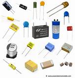
The next subject to be discussed in capacitance and the devices, capacitors. While resistors resisted the flow of electricity, capacitors actually store electrical energy, usually for very short periods of time. There are however, devices called super capacitors, that can store large voltages (but tiny current) much like batteries. They are very useful for powering circuits that may lose their primary power but can continue with voltage and low current, like CMOS circuitry which we will address later. Like resistors, capacitors come in a wide variety of types, values, accuracy tolerance, voltage, and current carrying capacities. When selecting a capacitor for use in a circuit, all of these must characteristics come into consideration, otherwise the circuit might not work, or worse, may be destroyed.
The figure below illustrates a few different types of capacitors. The capacitor may be made of air (separated by conducting metal plates), ceramic, plastic, glass, oil, tantalum, and probably more that I haven’t mentioned. Each material has different characteristics of determining capacitance and find preferred use in particular applications.
While the unit of measurement of the amount resistance is the ohm (Ω), the Farad is the unit of measurement of capacitance. A Farad is actually a huge amount of capacitance, most often we use millionth, billionth, or less values in circuits. A millionth (10-6) of a Farad is a microfarad (designated by µF or uF), a billionth is a nanofarad (nF or 10-9) while a trillionth is a pF or picofarad (10-12).
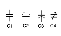
In the figure below, we can see several types of symbols that represent capacitors, C1 shows a non-polarized capacitor, typically made of ceramic, or plastic film. They are typically used to bypass noise to ground in power leads to semiconductors or power supplies, and in tuned circuits to perform timing or resonance when combined with a coil or resistor. C2 shows the symbol for a polarized capacitor which must be installed in a circuit with its + lead attached to a more positive lead and the other lead attached to a less positive component or lead. Failure to observe the correct polarity can result in the explosion of the capacitor. C3 is the more modern symbol for a polarized capacitor. C4 is a symbol of a variable capacitor, typically used in a tuned circuit to achieve resonance of the circuit over a range of frequencies. Variable capacitors are attached to the tuning dial of a radio to allow you to select the station you want to hear. Variable tuning capacitors typically use air as the non-conductive dielectric portion of the capacitor.
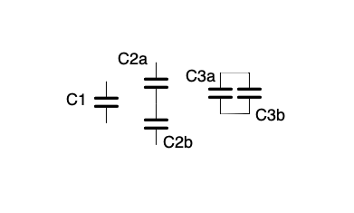
Capacitors can be arranged in either stand alone, series, or parallel configurations. However, the total capacitance exhibited by the combination is much different than when resistors are combined. Capacitors C2a and C2b in the figure below are series connected while C3a and C3b are parallel connected. Series connected capacitors add their values like parallel resistors. To compute the value of the combination of C2a and C2b, you would add 1/C2a and 1/C2b and then take the reciprocal of that total C = 1/(1/C2a)+(1/C2B). The value of parallel connected capacitors is C = C3a+C3b sort of like the combination of series connected resistors.
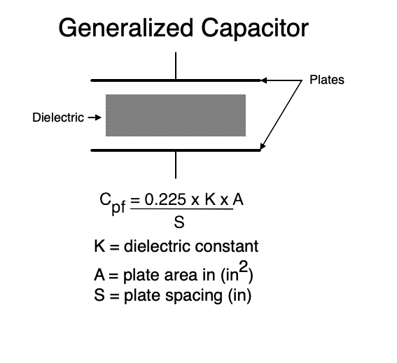
Below we have a diagram of a generalized capacitor. It is composed of two or more conductive plates separated by a dielectric material which may be only partially conductive. For instance, a non-conductive vacuum has a dielectric constant of 1.0 while air is 1.0006 and ceramic is 3-7. We see that the capacitance (in picofarads pF) can be roughly determined the area of the conductive plates multiplied by the dielectric constant of material between the plates all divided by the spacing between the plates. As the spacing increases, the capacitance decreases. As the dielectric constant or plate area increases, the capacitance increases.
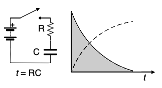
Now, let’s use a capacitor in a simple circuit containing a battery, a single pole switch, a resistor, and a capacitor. the instant the switch is closed, current starts to flow from the battery into the resistor and is limited by the resistor, and then into the capacitor. As shown in the grayed portion of the graph, voltage and current instantly goes from 0 to the maximum that can be supplied by the battery, then begins to decrease as the capacitor begins to charge then reach the full charge of the battery limited by the resistor (shown by the dashed line of the graph). At the point t on the Y time axis, voltage reaches maximum, and current minimum – the capacitor is fully charged. The time t that it takes to reach that point is called “time constant” and is computed by t = RC where R is the resistance in ohms (Ω) of the resistor and C is the capacitance measured in Farads of the capacitor.. If R = 1000Ω and C = .000001F or 1 uF or μF, t = 1000x.000001 = 0.001s or 1 millisecond.
Time constants are widely used in electronics, you will run into it many times. It is used to determine the frequency of oscillators, the timing of pulses, the resonant frequency of filters, many, many places.
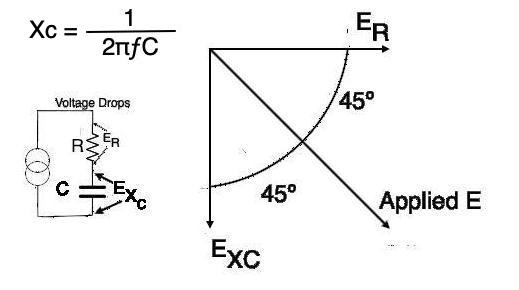
The flow of current (electrons) through a capacitor is dependent upon both the frequency of the alternating signal and the value of the capacitance. The greater the capacitance, the more electrons are required to bring the capacitor to fully charge to the source-voltage value. It is possible, in an AC circuit, to control the current flow by changing the capacitance just as a resistor controls the flow of current. The AC resistance effect is called capacitive reactance measured in ohms. Reactance is termed X while capacitive reactance is shown as Xc. The full formula is: Xc = 1/2πfC. We will encounter a different type of reactance again when we talk about inductors or coils. The higher the frequency or the higher the capacitance, the lower the total reactance because the formula is a reciprocal (divided by 1).
As we saw in the graph in the time constant illustration, it takes a finite amount of time for the capacitor to charge to the maximum amount of applied voltage. Similarly, it takes an amount of time for the capacitor to discharge once the applied voltage is removed. This delay in charging and discharging causes a phase shift from the original applied signal. Again, referring to the graph, we see that the applied current instantly reached maximum but then tapered off as time progressed. Conversely, we saw that the applied voltage took some time to increase to its maximum level. So voltage lags current, or current leads voltage by some amount of delay. In a purely capacitive circuit (no resistance) that voltage delay will be by 90º, decreasing to 45º as the circuit resistance approaches the value of capacitive reactance.
Capacitors are not perfect. They have some amount of intrinsic resistance in them dues to their leads and dielectric losses. This resistance contributes to the slight phase lag through the component and may be added to the external, much larger resistance. This intrinsic resistance is called ESR or equivalent series resistance. ESR is an AC measurable phenomenon, not DC, and increases with frequency. ESR is much lower in ceramic and plastic film capacitors, and much higher in electrolytic and tantalum capacitors. The much higher ESR in electrolytics can become a problem with age. The dielectric dries out with time and can raise the ESR to a point that it causes excessive internal heating of the capacitor and even catastrophic failure of the component.
This section will introduce you to the simplest of electronic components, the resistor. There are many forms of resistors to suit the intended application.
If an EMF (electromotive force) or voltage can flow from one point to another, the material it is flowing through is termed a conductor. If, on the other hand, no EMF flows, the material is termed an insulator. The best conductor is gold, next silver, then copper, and aluminum. The best insulator is glass and ceramic, other insulators like rubber, plastic, and paper are used to isolate conductors. As conductors increase in length, their resistance also increases.
Resistors are used to impede the flow of current or voltage, and to interact with other components like capacitors and sometimes inductors to create turned circuits.
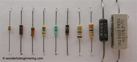
Resistors come in a very wide variety of types and forms, from devices that measure light and heat and sound, to devices that control audio loudness, to devices that control light, heat, and power. Resistors can be made of lengths of wire, carbon powder compressed into tubes, and metal foil, oxide, or vapor sintered onto insulating forms. Most often, when building electronic circuits, I use metal film resistors. They are daily temperature stable, lower noise generating than carbon, available is several power ratings and accuracies, and are low cost. Interestingly, it is difficult to predict the final resistance of a manufactured resistor so these days, the process is more one of a measuring and sorting operation. Manufactured resistors are measured then sorted into batches of similar devices that are all within 1%, 5%, or 10% of the intended value. Just a few are shown in the illustration below.
The values of resistors are measured in ohms. Resistors range in values from 1/1000th of an ohm to many millions of ohms. The most common values that you will use and run into range from about .5 to 1,000,000Ω. The higher and lower values are used for special purposes. Besides the value of resistance of the component itself, you will need to know and consider its power value and component accuracy. The most common power values are 1/4, 1/2, and 1 watt values. Smaller and much larger power handling capability are also available. The most common accuracy values are 1%, 5%,and 10% although much more precise accuracies are available for special purposes.
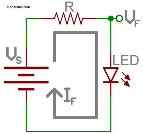
To determine the power value of the resistor you intend to use, you need to know the ranges or voltage or current that will flow through the resistor, then use the variants of Ohm’s Law to determine the power rating. For example, ass Ume you need a resistor to limit the current flow to an LED in a circuit that has 12 volts available. The resistor’s value will need to be (12V – (1.2Vf of the LED – the forward voltage drop across the LED) = 10.8V) x (.020 A for normal brightness) = 10.8/0.020 = 540Ω. The nearest standard value, not exceeding the required 0.02A of current) is 560Ω. Now, to determine the power rating of the 560 ohm resistor we square the current and multiply by the resistance: I2xR = .0004×560 = .224W which is a little too close to 1/4W so best to use 1/2W power rating so it won’t overheat with the current flowing through it. See the illustration below.
The ohmic value, accuracy, and power handling capability of most resistors can be identified by a color code imprinted on the body of the component. The code may be memorized by: BROYGBVGWB. Which stands for Brown, Red, Orange, Yellow, Green, Blue, Violet, Gray, White, Black; 1,2,3,4,5,6,7,8,9,0. A resistor with a color code of Brown, Green , Yellow would have the digits 15 then the number of zeros to add to the first two digits. The third ring of yellow indicates 4 zeros to add to the resistor’s value so the final value would be 150,000. Similarly a fourth ring indicates the accuracy tolerance: gold, 5%, silver, 10%. Power handling is usually indicated by size: the smallest is usually 1/10W, next 1/4W, then 1/2W, 1W, 5W, 10W, 50W. The larger resistors, usually larger than 1/2W, will have the power value printed on the body of the component.
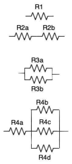
Several resistors are shown the the figure above. The symbol used on schematic diagrams of a circuit is shown as R1. If two resistors are connected in series, they are shown as R2a and R2b. Resistors connected in parallel are shown as R3a, R3b, and R3c. Finally, if resistor combinations are connected in series and parallel, they may be shown as R4a, R4b, R4c, and R4d. There can be many combinations of all these types of connections.
When resistors are connected in series, as shown by R2a and R2b, the total resistance of the combination is the sum of each of the individual resistors in the network. For example, if Ra = 150 ohms, and Rb is 400 ohms, the series combination is 150+400 = 550.
When resistors are connected in parallel such as R3a and R3b, the combined network is a bit different: it is: 1 / 1 / R3a + 1 / R3b. If R3a = 100 ohms, and R3B is 500 ohms, the parallel combination shown is 1 / .01 + .002 = 1/.012 = 83.33. If all the resistors connected in parallel are of the same value, you may calculate the network as a special case as R1xR2/R1+R2. For example if R1=R2=100 ohms, the parallel combination of the two in parallel would be 100×100/200 = 50.
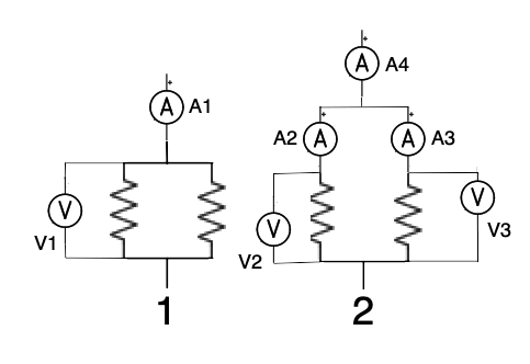
Voltage is a circuit is measured across one or more components, while current is measured within a circuit. In the circuit below (part 1), we see that a voltmeter is applied across the resistor network, which the ammeter is applied within the circuit. Lets assume that the voltmeter reads 100V in this circuit while one resistor has a value of 100 ohms, and the other has a value of 800 ohms. The parallel circuit of the two resistors (in part 1) is 1/1/100+1/800 = 88.88 ohms of resistance. When placed in a 100V circuit, by Ohm’s law, we see that E/R = I and thus 1.125 amps of current would be shown by the ammeter A1.
In the illustration’s part 2, we have added a couple more meters to see that the voltage across the two resistors as measured by meters V2 and V3 both still read 100V, just as did V1 in part 1. However, we can see that “current divides” in the two parallel resistors. A2, the ammeter in the 100 ohm resistor circuit will read 1.0 amp while the ammeter A3 will read 0.125 amps.. A4, the ammeter reading the current for the entire parallel resistor circuit will still read 1.125 amps. We see that current divides in parallel circuits, voltage does not.
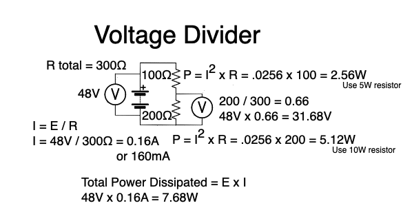
Now, let’s consider a commonly encountered circuit construct called a voltage divider. A voltage divider is used to obtain a lower voltage from a higher voltage. It is composed of resistor networks (either series or parallel combinations or both) and a higher voltage source than you wish to obtain. The voltage divider is shown in the illustration below.
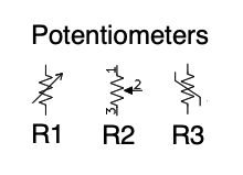
There are several other critical components that are based upon the simple resistor. One of the simplest is the potentiometer or pot, really a variable resistor. The devices have three terminals, two are just like a fixed resistor, the third is like the voltage takeoff terminal we saw in the voltage divider. Three different symbols for potentiometers are shown below. The center one, R2, illustrates the three terminals. Terminal 2 is the “take off” pin for the variable resistance between terminals 1 and 3. The fixed portion is between terminals 1 and 3, the variable resistance is between terminals 1 and 2, or 2 and 3, depending upon how you want the circuit to work. That variable resistance appearing at terminal 2 is usually determined by the rotary position of a control knob, or the vertical position of a slider. Varying the position of the knob or slider changes the resistance appearing at that variable terminal. There are many uses for such a device.
In addition to pots, variable resistors are used to detect changes in temperature (termed thermistors), light (termed photocells), or sound (termed electret microphones). There are probably others.
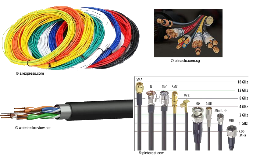
Most wire used in electronics is made of copper due its low resistance. Some aluminum is also used. Wire may be stranded from smaller gauges of wire to make it flexible, or drawn into a solid single conductor which is stiffer than stranded. Household electrical wiring is usually 12 or 14 AWG (American Wire Gauge). Wire may be insulated with enamel, plastic, vinyl, or fabric or may be bare, without insulation. Wire may be straight or coiled, commonly used to connect microphones.
Most wire used to hook up circuits on boards or between boards, use 18 through 24 AWG insulated stranded or solid in a variety of colors. Several wires joined together in a common insulating jacket it termed a cable. One form of cable commonly used in amateur radio is coax. Coax varies in its diameter, larger versions having greater power carrying capacity than the thinner ones. Coax is designated by an abbreviation, RG, followed by an identifying number. RG-174, about the smallest commonly encountered in amateur radio is about the same diameter as 12AWG electrical wire. The next size up, RG-58 (or RG-59 used for TV connections) is usually used to connect receivers to antennas. RG-8 an even thicker cable capable of handling up to 1000W, is used for low resistance connections from transmitters to antennas (and receivers as well).
There are larger versions of coax, often termed hardline because they have a rigid outer conductor or shield. Hardline is very expensive and requires special connectors and installation techniques, however it can handle the carriage of enormous amounts of power – it is most often used in commercial broadcast operations.
Remember our friend E = IR? Well that equation works perfectly well for DC circuits, those most commonly found in electronics. However, that simple equation doesn’t actually suffice for AC circuits. Both frequency and phase come into play when computing values in AC circuits.
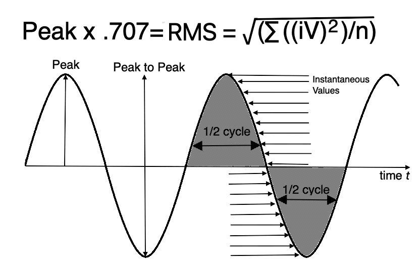
If we take the value of the peak of an AC waveform and multiply it by 0.707 we will have the RMS or effective value of the waveform. The RMS value is the portion of the AC waveform that can do actual work (the portion of the drawing that is grayed out). RMS means root-mean-square. It is the square root of the average (or mean) of the sum of the squares of the instantaneous values of the voltage or current.
The RMS value of an AC waveform is equivalent to the peak value of a DC waveform. DC waveforms don’t really have peaks, it is a constant value. To determine the value of AC that is equivalent to DC, we need to multiply the AC effective value by 1.414 (the reciprocal of .707 or 1/.707).
When problems are given to be solved, it is presumed that the effective value is to be employed. For instance, when the power company states that it is supplying 120VAC it means 120 Veff which is 120 x 1.414 or about 170V peak.
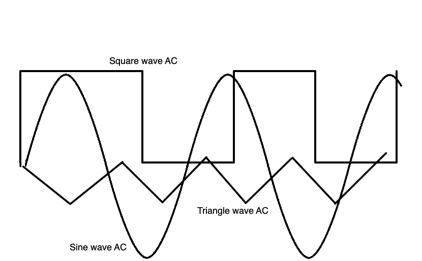
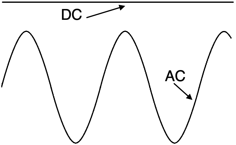
Recall from the section on DC that the direct current flow does not reverse direction or is interrupted in time. On the other hand, AC or alternating current, does reverse direction, from positive to negative, or from positive to less positive, or negative to less negative. Alternating current propagates through wires with less resistance (hence power loss through heat) than does DC. AC power transmission allows there to be much greater distances between the point of power generation to the point of power consumption. An epic struggle of philosophy occurred in the late 1800’s between Thomas Edison (proponent of DC and inventor of the modern light bulb) and Nikola Tesla (proponent of AC power distribution). Tesla won that battle, principally because of cost. AC power is less expensive to transmit long distances than DC. Though AC is useful for direct use as a source of power for heating and lighting, DC is the preferred power source for most electronics. AC is easily converted to DC with just a few components while converting DC to AC requires a bit more trouble and circuitry.
Current performs the work of electricity. Voltage is the pressure applied to the current. Alternating current or AC reverses direction of flow, from negative to positive, then positive to negative. How often this reversal occurs per second determines the frequency of the alternation. If only one reversal per second occurs, the frequency is 1 Hz (Hertz is the name for frequency instead of Cycles Per Second – CPS – from years ago). If the reversal occurs 60 times per second, the measurement is 60 Hz. Ranges of frequencies have been characterized as “spectrum bands”. 0 to 30,000 Hz (0 to 30 KHz, Extremely, Super, Ultra, Very, and Low Frequency) is considered to be the audio spectrum; 30,000 (30 KHz) to 300,000 (300 KHz) Hz is called Low Frequency (LF); 300,000 (300 KHz) to 3,000,000 (3 MHz) is called Medium Frequency radio frequency (MF) spectrum; 3,000,000 to 30,000,000 (3 MHz) to 30 MHz) is called High Frequency (HF) RF; 30,000,000 (30 MHz) to 300,000,000 (300 MHz) is called Very High Frequency (VHF); 300,0000,000 (300 MHz to 3,000,000,000 (GHz) is called (Ultra High Frequency UHF). Higher frequency bands have similar names.
There are three types of frequency measurement: rotational, angular, and spatial. Rotational frequency usually denoted by the Greek letter ν (nu), is defined as the instantaneous rate of change of the number of rotations N, with respect to time: ν = dN/dt; it is a type of frequency applied to rotational motion. Angular frequency usually denoted by the Greek letter ω (omega), is defined as the rate of change of angular displacement (during rotation), Θ (theta), or the rate of change of the phase of a sinusoidal waveform (notably in oscillations and waves), or as the rate of change of the argument of the sine function:
ƒ = 1/T (oscillation, waves, or harmonic motion)
ω = 2πƒ (angular frequency in radians)
ν = dN/dt (rotational frequency)
k = 2π/λ or 2πξ where (ξ=1/λ) (spatial frequency)
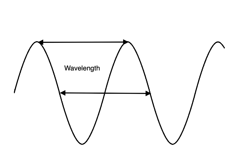
The frequency of AC is measured through one complete cycle, from positive peak to positive peak, or negative peak to negative peak, or from when the signal passes through the 0 Y axis to the next time it passes through that axis.
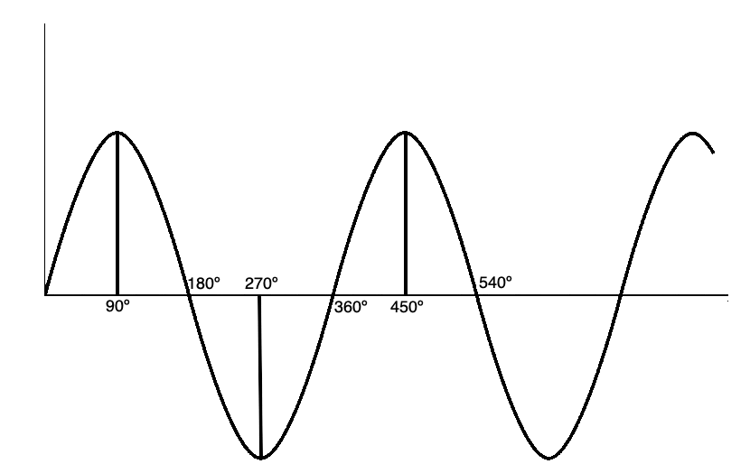
As one cycle completes, it passes through 360 angular degrees of phase. One positive peak, or one negative peak completes 180 degrees of angular phase. The phase measured from the point the wave passes through the 0 Y axis to the next peak is 90 degrees of phase angle.
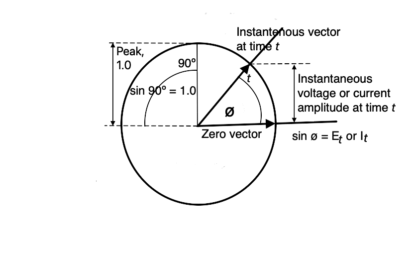
Rotating vectors can be used to indicate the instantaneous value of voltage or current. The rational distance between the zero vector and the instantaneous vector length (from 0.0 to 1.0 if the rotational angle is less than or equal to 90º, or 0.0 to -1.0 if the rotational angle is greater than 90º) of the signal under measurement is equal to the sin of the rotational angle times the peak value.
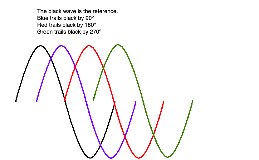
Phase is measured from a starting point on the waveform, usually the crossing point of the 0 point of the Y axis. We will define that point as 0º. As the waveform progresses in time, we pass through 90º at the first peak, then 180º at the next crossing of the 0 point of the Y axis, then 270º at the negative peak, and finally the 0 crossing point of the Y axis agin. We’ve completed a full 360º of phase transition.
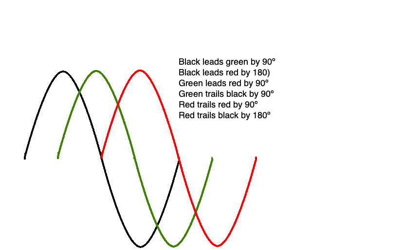
The phases of two of more signals may be compared from their individual 0 Y axis crossing points. If the black wave is our reference wave, the other colors of waves cross the 0 Y axis at different times, leading or lagging the reference crossing of the black trace.
Magnetism is a physical property that certain materials posses that permits them to attract or repel similar or other materials that exhibit magnetism. Magnetism and electricity are intertwined. Electricity can generate or alter magnetism, magnetism can generate or alter magnetism. Hence the term “electromagnetism” is used to describe the conjoined phenomena.
Magnetism itself cannot be seen, but the effects of it are readily apparent. Sprinkling iron filings on a page of paper that has a magnet placed beneath the paper shows the magnetic field near the magnet can align and attract the iron filings on the face of the paper. Holding a magnet near another magnet or a piece of magnetic material such as a small iron plate, will show that an attraction or repulsion between the two items may begin a bit of a ways from each other without the items actually touching. The effect reveals that there is an invisible magnetic field around the magnet. Passing other “magnetic materials” through that field can result in the generation of electricity. Similarly, winding a length of wire into a coil around an iron nail and connecting the ends of the wire to the terminals of a current source such as a battery will produce a magnet out of the nail allowing it to attract other nails. These properties of electromagnetism are found in thousands of electronic devices that are used to improve our lives. Using your LEFT hand, point your thumb straight out to indicate the direction of the flow of a current. The fingers wrapped around then indicate the direction of the magnetic field lines of force. This is known as the left hand rule of magnetism.
Several characteristics of magnetism need to be described at this point that will later be necessary to understand the purpose and performance of certain electronics devices used in the circuitry of electronics and radio. The lines of magnetic force (or magnetic field) is designated as ø. If 100 lines of force are produced in a coil, ø=100. If the cross sectional area of the coil is 2 in2 then the flux density, designated by the symbol B, is 100/2 = 50 (B =ø/d). The intensity of the magnetic field is termed magnetomotive force or MMF. MMF may be computed by multiplying the number of turns in the coil by the current flowing through the wire, F = NI. Either increasing the number of coil turns or increasing the current in the coil or both will increase the strength of the magnetic field produced. The magnetization vector is the distribution of magnetic moments in the region. The symbol dm is the magnetic moment, dv is the volume element.
Magnetic field intensity is represented by the symbol F. If a 3 inch coil with 60 amp-turns (2 amps x 30 turns in the coil) has a field intensity of 60/3 = 20. The field flowing from a wire or coil of wire are pushed back by air but when a piece of iron is introduced into the magnet field, the density of lines of force (or flux) will increase. The iron expands the flux from the wire outward and concentrates the flux. In other words, the magnetic flux density increases. If a wire with a current of 1 amp flowing is turned into a 1 inch diameter coil having 20 turns, a flux density of 20 lines/in2 will be created. If, however, we wrap that wire coil of 20 turns around a nail, a flux density of perhaps 200,000 lines/in2 may be created.
Finally, permeability (a variant of the word permeate or saturate, not the word permanent) represented by the symbol µ, is the ability of as core material to be permeated by lines of force. The permeability of air may be assumed to be 1. Materials such as iron, nickel, and cobalt are highly permeable and have values of hundreds to thousands of times that of air.
These are the equations you need to be familiar with from this section:
ø = Bd for magnetic flux measured in Webers
B = ø/d for magnetic flux density measured in Tesla
M = dm/dv magnetization vector measured in Amperes per meter A/m
H = 1/µB-M magnetic field intensity measured in Ampere per meter A/m
F= NI for MMF intensity measured in Amperes
µ = B/H or µ(H+M) for permeability measured in Henrys per meter h/m
Magnetism has been known of for thousands of years since discovering that certain rocks (lodestone) could attract iron. Compass needles were originally magnetized by rubbing them on lodestone then floating the needle in water to permit it to point north thereby allowing marine navigation out of the sight of land references. Study of magnetism progressed from the ancient world up until 1819 when Hans Christian Orsted discovered that a compass needle would respond when an electric current passing through a closed loop of wire was passed near the needle. Soon, in 1831, Michael Faraday discovered that when passing a loop of wire through a magnetic field, an electric current was produced. James C. Maxwell then describe this phenomenon and tied it together with electricity, magnetism, and optics (he proposed that light is an electromagnetic phenomena). Maxwell’s equations together define the speed of light (as “c”, a constant speed in a vacuum at 299,792,458 meters per second or 186,263.7559 miles per second). The speed of propagation in a vacuum is the fastest that electricity can travel, that speed is somewhat less when traveling in wire. Some wire, especially coax, is specified with a velocity factor indicating how much more slowly that electricity will travel. Velocity factor becomes important when computing the length of wire to use in resonant or tuned circuits for radio. In 1905, Albert Einstein used Maxwell’s equations to describe the special theory of relativity. When electromagnetic phenomena are propagated through wires, air, or empty space, it is called radiation. As waves of electromagnetic radiation they occur at various wavelengths to produce a spectrum from radio waves to gamma rays.
Faraday’s discovery of the ability to create electricity by passing a wire through a magnetic field resulted in the first hydroelectric power generators that allowed large scale electricity production by attaching rotating coils of wire attached to a shaft placed in a stationary magnetic field together at hydroelectric dams, coal fired steam generators, and eventually nuclear powered generators to feed a grid of wire distributing electricity to all of civilized society. Conversely, when electricity is applied to the coil with rotating magnets attached to a shaft, we have a motor. Generators can drive motors, motors can drive generators. We use both now every day.
Electromagnetism is used in many aspects of modern electronics. A relay uses an electromagnet to close a switch to control another device or signal the state of another device. A variant of a relay is a buzzer used for audible signaling. Still another variant called a solenoid causes movement in an arm that can open and close doors, valves, and other things. A speaker converts varying electric currents to sound by using an electromagnet to move a cone of paper or plastic to create a sound wave. A microphone converts sound to a varying electric signal by the same approach. A device called an inductor or transformer (a coil of wire sometimes wrapped around a magnetic core) to slightly delay a varying electric signal in time. That delay only occurs with varying electric signals, not direct current signals. That characteristic, combined with a similar varying electric signal delay caused by devices called capacitors results in combinations of those two devices to create tuned circuits that can be used to select only certain signals meeting desired ranges of frequency to be passed through the circuit (more on tuned circuits later).
Understanding and using electronics will involve mathematics. It is completely unavoidable. Math and electronics are intertwined, as are all of the sciences: physics, chemistry, biology, astronomy. Its what the sciences are: understanding and describing and predicting the natural processes and phenomonen with mathematics. If you are interested in electronics, you will have to obtain some level of expertise in math. To begin with, our friend Ohm’s Law and relatively simple algebra will get you started. Using algebra will allow you to comprehend and understand the behavior of DC electricity and eventually AC, radio, electrooptics, microwave, cell phones, and television. Let’s get started.
Recall now what you learned from the section of this blog titled “Current”. Current is defined as the flow of electrons from a point of negative charge (meaning a point of higher density of electrons) to a point of lesser density of electrons. The lesser density point need not be “positively” charged, only less negative than the other point. A current, or flow of electrons, will occur because the difference in charges is seeking to even itself out, to obtain a charge differential of zero.
If the transfer or flow of electrons occurs without interruption in time, and without reversal of direction, it is termed direct current or dc or DC. The flow may occur at any voltage greater than zero. There needs to be a voltage differential greater than zero else the current cannot flow. The current section below describes the amount of charge flow required in one second to constitute a single amp of current. That current may be measured in units, tens, hundreds, thousands, or more, or in tenths, hundredths, or thousandths, millionths of an amp. Amp is the shortened name for Ampere. If the measurement involves thousandths of an amp, we term the measurement is in milliamps, abbreviated ma. If millionths of an amp, we use the term microamps and the abbreviation ua or µa. There are one thousand microamps in a single milliamp. Likewise, there are one thousand milliamps in a single amp.
If the DC current flow is interrupted, particularly at a regularly timed rate, it is termed pulsed DC. The pulses may vary at a relatively slow rate, maybe once or twice per second, or at a very fast rate, perhaps hundreds, thousands, or millions of times per second. As long as the pulses vary their voltage from zero to a positive or negative value, the current stream is considered to be pulsed DC. If the current varies from a positive value to a negative value, and back to a positive value, it is considered to be alternating, not pulsed. The nuances here will become important later on.
DC current was the second type of electricity to be generated on demand, the first was static electricity generated by rubbing materials with fur or fabric. DC was created within devices we now call batteries using chemical reactions between dissimilar materials and compounds. The first individual to do that was Alessandro Volta in 1800. Those early devices were named after him and termed voltaic piles.
The ability to generate electricity on demand using voltaic piles greatly stimulated the study of electricity and its properties. Throughout the early and mid 1800’s, physicists, chemists, and scientists were able to replicate and verify each others discoveries about the properties of electricity.
Today, most electronic devices utilize DC in some particular way. Useful voltages ranging from about 1.5 volts produced by simple carbon or alkaline batteries through 3.3 volts used by modern electronics in cell phones to 5 volts used by most computers to 12 volts used by most modern cars all rely on DC. Some railroads and most subways utilize very high DC currents to drive their motors at voltages from 750 to 3000 volts. The first practical incandescent electric lights developed by Thomas Edison in the late 1800’s also utilized DC. DC however is difficult to transmit over long distances. The primary advisary of Edison was Nikola Tesla who was a proponent of alternating current, AC, and participated in bitter arguments with Edison and his DC electricity distribution. Edison, known for the invention of many things including the phonograph and moving pictures, was wrong about the practicality of wide-scale distribution of DC for electric lighting purposes. Tesla’s AC eventually dominated and replaced Edison’s DC as a more efficient alternative. Today, we have the benefit of using both and can easily convert the AC transmitted from far away generators to DC to power our electronic devices.